Other Good Blogs & Scripts

Script Location from ORACLE-BASE


http://oracle-base.com/dba/scripts.php
.
--- Blogs ---




http://pjacksondba.blogspot.com/

http://tkyte.blogspot.com/

http://blog.tanelpoder.com/

http://jonathanlewis.wordpress.com/

http://carymillsap.blogspot.com/

http://karenmorton.blogspot.com/




Database Server Upgrade/Downgrade Compatibility Matrix (Doc ID 551141.1)
Patching & Maintenance Advisor: Database (DB) Oracle Database 11.2.0.x (Doc ID 331.1)
Oracle Recommended Patches -- Oracle Database (Doc ID 756671.1)
Introduction to Oracle Recommended Patches (Doc ID 756388.1)
Oracle Recommended Patches (PSU) for Enterprise Manager Base Platform (All Releases) (Doc ID 822485.1)
-- For Upgrade and Install
Oracle® Grid Infrastructure Installation Guide 12c Release 1 (12.1) for Microsoft Windows x64 (64-Bit)  E49041-03
-- Oracle Database Online Documentation 12c Release 1 (12.1)
https://docs.oracle.com/database/121/nav/portal_11.htm
Oracle® Grid Infrastructure Installation Guide 11g Release 2 (11.2) for IBM AIX on POWER Systems (64-Bit) E48294-01
Oracle® Grid Infrastructure Installation Guide 12c Release 1 (12.1) for IBM AIX on POWER Systems (64-Bit)
-- For Upgrade and Install
http://mirrors.iyunwei.com/oracle/docs/12.1-E16655-01/install.121/e38943.pdf
--
Oracle Database 12c R1 RAC on IBM AIX
http://www-03.ibm.com/support/techdocs/atsmastr.nsf/5cb5ed706d254a8186256c71006d2e0a/781e2275188c706886257c98006b1c6e/$FILE/IBM%20AIX%20Oracle%2012cR1-tips_SHANMUGAM%2026%20Feb%202014.pdf
--
http://docs.oracle.com/database/121/nav/portal_booklist.htm

Useful Queries

========================================================

Constraints Queries
========================================================


select 'alter table '||a.owner||'.'||a.table_name||' disable constraint '||a.constraint_name||';'
from all_constraints a, all_constraints b
where a.constraint_type = 'R'
and a.r_constraint_name = b.constraint_name
and a.r_owner  = b.owner
and b.table_name = 'Table Name Here'
/
-- generic

select CONSTRAINT_NAME,OWNER,TABLE_NAME,STATUS
from DBA_CONSTRAINTS
where R_CONSTRAINT_NAME
in
( select CONSTRAINT_NAME
  from dba_constraints
  where TABLE_NAME in ('MASTER') 
)
/ 

-- Get Columns (Generic Query)

select * from DBA_CONS_COLUMNS
where (CONSTRAINT_NAME,OWNER,TABLE_NAME)
in
( select CONSTRAINT_NAME,OWNER,TABLE_NAME 
  from DBA_CONSTRAINTS
  where R_CONSTRAINT_NAME
  in
  ( select CONSTRAINT_NAME
    from dba_constraints
    Where  TABLE_NAME in ('MASTER')
  ) 
)
/ 

========================================================
-- session/process info
========================================================


select *
from  gv$session s, gv$process p
where s.paddr = p.addr
and   s.inst_id = p.inst_id
--and s.sid='5552'
;

select  s.inst_id
       ,s.STATUS
       ,s.sid
       ,p.spid
       ,substr(s.username,1,15) usernm
       ,substr(s.program,1,15) program
       ,substr(s.MACHINE,1,15) machine
       ,substr(s.TERMINAL,1,15) terminal
       ,substr(s.MODULE,1,15) modul
       ,substr(s.ACTION,1,15) action
       ,s.LOGON_TIME
       --,p.PGA_USED_MEM
       --,p.PGA_MAX_MEM
       ,s.SQL_HASH_VALUE      
       ,s.BLOCKING_SESSION
       ,command
from
   gv$session     s,
   gv$process     p
where s.paddr = p.addr
and   s.inst_id =p.inst_id
--and   s.username is not null
--and s.username='ADARSHKUMAR'
--and s.module not like '%Apol%'
--and status ='ACTIVE'
--and blocking_session is not null
--and s.MACHINE not like '%web%'
--and s.MACHINE not like '%beta%'
--and s.MACHINE not like '%seci%'
--and s.sid =4
order by 3  
;




=======================================================
-- Wait Event Queries
========================================================
select wait_class_id, wait_class, count(*) cnt
from dba_hist_active_sess_history
where snap_id between 21277  and 21285
group by wait_class_id, wait_class
order by 3;

- Use Classid and Look the Enets whit Higher  Count


select event_id, event, count(*) cnt
from dba_hist_active_sess_history
where snap_id between 21281 and 21285
and wait_class_id=3871361733
group by event_id, event
order by 3;


------------------------------
- Now Get The SQL Statement
------------------------------
select sql_id, count(*) cnt
from dba_hist_active_sess_history
where snap_id between 21281 and 21285
and event_id in (1478861578, 2701629120)
group by sql_id
having count(*) > 1
order by 2;

- Go for SQl
--- Max cnt 871



select sql_text
from dba_hist_sqltext
where sql_id='$id';

========================================================
  -- Hot Block Query
========================================================


SELECT SEGMENT_NAME, SEGMENT_TYPE
FROM DBA_EXTENTS           
WHERE FILE_ID = &fileid  AND &block  BETWEEN BLOCK_ID AND                 
BLOCK_ID + BLOCKS - 1; 


-----------------------------------------
-- Check who is blocking and How may sessions are affected
-- This session needed to be killed
-----------------------------------------

SELECT blocking_sid, num_blocked
FROM ( SELECT blocking_sid, SUM(num_blocked) num_blocked
       FROM ( SELECT l.id1, l.id2,
               MAX(DECODE(l.block, 1, i.instance_name||'-'||l.sid,2,i.instance_name||'-'||l.sid, 0 )) blocking_sid,
               SUM(DECODE(l.request, 0, 0, 1 )) num_blocked
               FROM gv$lock l, gv$instance i
               WHERE ( l.block!= 0 OR l.request > 0 ) AND
               l.inst_id = i.inst_id
                GROUP BY l.id1, l.id2
              )
        GROUP BY blocking_sid
        ORDER BY num_blocked DESC
      )
WHERE num_blocked != 0;

-----------------------------------------------------------
-- check who has locked the object
-----------------------------------------------------------
select * 
from gv$locked_object
where object_id in ( select object_id from dba_objects where object_name='TEST');


-- Detail of above Query
select p.spid,s.*
from gv$session s,
     gv$process p
where s.paddr=p.addr
and   s.inst_id = p.inst_id
and s.sid in ( select k.session_id 
                   from gv$locked_object k
                   where k.object_id in ( select object_id from dba_objects where object_name='&TABLE_NAME')
                   and s.inst_id = k.inst_id
                 );


-- Find SQL Associated
select * from gv$sqlarea where sql_id='&SQL_ID';

===================================
Transaction Queries
===================================




Check who is using most REDO and If  it is still Rolling Back


SELECT s.inst_id,s.username,s.schemaname,s.osuser,s.machine,s.program,
       s.sid,
       s.serial#,
       t.used_ublk,
       t.used_urec,
       rs.segment_name,
       r.rssize,
       r.status
FROM   gv$transaction t,
       gv$session s,
       gv$rollstat r,
       dba_rollback_segs rs
WHERE  s.saddr = t.ses_addr
AND  t.inst_id=s.inst_id
and  s.inst_id=r.inst_id
AND    t.xidusn = r.usn
AND   rs.segment_id = t.xidusn
ORDER BY t.used_ublk DESC
/

-- Find when Transaction started for a specific table
-- and Check the Current Status

select * from 
GV$TRANSACTION
where (XIDUSN,XIDSQN,XIDSLOT) in 
( 
select XIDUSN,XIDSQN,XIDSLOT 
from gv$locked_object
where object_id in ( select object_id from dba_objects where object_name='&table_name_here')
);

SELECT start_timestamp,commit_timestamp,logon_user,table_owner,table_name,operation, undo_sql
FROM flashback_transaction_query ftq,v$transaction vt,v$session vs
WHERE ftq.xid = vt.xid and vt.ses_addr=vs.saddr AND vs.sid =&SID;


-- chk spid  and other info
select  s.inst_id
       ,s.STATUS
       ,s.sid
       ,p.spid
       ,substr(s.username,1,15) usernm
       ,substr(s.program,1,15) program
       ,substr(s.MACHINE,1,15) machine
       ,substr(s.TERMINAL,1,15) terminal
       ,substr(s.MODULE,1,15) modul
       ,substr(s.ACTION,1,15) action
       ,s.LOGON_TIME
       ,p.PGA_USED_MEM
       ,p.PGA_MAX_MEM
       ,s.SQL_HASH_VALUE      
       ,s.BLOCKING_SESSION
       ,command
from
   gv$session     s,
   gv$process     p
where s.paddr = p.addr
and   s.inst_id =p.inst_id
--and s.username='ADARSHKUMAR'
--and s.module not like '%Apol%'
--order by status,inst_id,sid
order by PGA_USED_MEM desc
;

========================================================
 -- Temp Space Usage  Queries
========================================================


select * FROM gV$SORT_SEGMENT;

select a.inst_id,b.sid, a.session_num serial# , a.username,
       a.segtype,
       to_char(a.blocks*16/1024,'999,999,999,999')  space_used_MB ,
a.SQLHASH ,a.SQL_ID ,a.TABLESPACE,
trunc((blocks*16*1024/tot) *100,1) || '%' as pct_used
from gv$sort_usage a,gv$session b,(select sum(blocks*16*1024) tot
                     from gv$sort_usage su
                     ) n
where a.inst_id = b.inst_id
and   a.session_num = b.serial#
order by a.blocks desc;

select b.machine,a.inst_id, a.username, a.segtype,
       to_char(a.blocks*16/1024,'999,999,999,999') space_used_MB ,
       a.SQLHASH ,a.SQL_ID ,a.TABLESPACE,
trunc((blocks*16*1024/tot) *100,1) || '%' as pct_used
from gv$sort_usage a,gv$session b,(select sum(blocks*16*1024) tot
                     from gv$sort_usage su
                     ) n
where a.inst_id = b.inst_id
and   a.session_num = b.serial#
order by a.blocks desc;

========================================================
Redo Space Usage Queries

========================================================

-- Size of log generated


select dest_id,trunc(COMPLETION_TIME) TIME,
to_char(trunc(SUM(BLOCKS * BLOCK_SIZE)/(1024*1024)),'999,999,999') SIZE_in_MB ,count(*) cnt
from gV$ARCHIVED_LOG
--where COMPLETION_TIME > sysdate -10
where inst_id =1
group by dest_id,trunc (COMPLETION_TIME)
order by 2 desc,1;



=====================================================================
log switches per hrs / Archive Logs History
 
=====================================================================

SELECT * FROM
(
SELECT * FROM ( SELECT TO_CHAR(FIRST_TIME, 'DD/MM') AS "DAY" ,
SUM(TO_NUMBER(DECODE(TO_CHAR(FIRST_TIME, 'HH24'), '00', 1, 0), '99')) "00:00" ,
SUM(TO_NUMBER(DECODE(TO_CHAR(FIRST_TIME, 'HH24'), '01', 1, 0), '99')) "01:00" ,
SUM(TO_NUMBER(DECODE(TO_CHAR(FIRST_TIME, 'HH24'), '02', 1, 0), '99')) "02:00" ,
SUM(TO_NUMBER(DECODE(TO_CHAR(FIRST_TIME, 'HH24'), '03', 1, 0), '99')) "03:00" ,
SUM(TO_NUMBER(DECODE(TO_CHAR(FIRST_TIME, 'HH24'), '04', 1, 0), '99')) "04:00" ,
SUM(TO_NUMBER(DECODE(TO_CHAR(FIRST_TIME, 'HH24'), '05', 1, 0), '99')) "05:00" ,
SUM(TO_NUMBER(DECODE(TO_CHAR(FIRST_TIME, 'HH24'), '06', 1, 0), '99')) "06:00" ,
SUM(TO_NUMBER(DECODE(TO_CHAR(FIRST_TIME, 'HH24'), '07', 1, 0), '99')) "07:00" ,
SUM(TO_NUMBER(DECODE(TO_CHAR(FIRST_TIME, 'HH24'), '08', 1, 0), '99')) "08:00" ,
SUM(TO_NUMBER(DECODE(TO_CHAR(FIRST_TIME, 'HH24'), '09', 1, 0), '99')) "09:00" ,
SUM(TO_NUMBER(DECODE(TO_CHAR(FIRST_TIME, 'HH24'), '10', 1, 0), '99')) "10:00" ,
SUM(TO_NUMBER(DECODE(TO_CHAR(FIRST_TIME, 'HH24'), '11', 1, 0), '99')) "11:00" ,
SUM(TO_NUMBER(DECODE(TO_CHAR(FIRST_TIME, 'HH24'), '12', 1, 0), '99')) "12:00" ,
SUM(TO_NUMBER(DECODE(TO_CHAR(FIRST_TIME, 'HH24'), '13', 1, 0), '99')) "13:00" ,
SUM(TO_NUMBER(DECODE(TO_CHAR(FIRST_TIME, 'HH24'), '14', 1, 0), '99')) "14:00" ,
SUM(TO_NUMBER(DECODE(TO_CHAR(FIRST_TIME, 'HH24'), '15', 1, 0), '99')) "15:00" ,
SUM(TO_NUMBER(DECODE(TO_CHAR(FIRST_TIME, 'HH24'), '16', 1, 0), '99')) "16:00" ,
SUM(TO_NUMBER(DECODE(TO_CHAR(FIRST_TIME, 'HH24'), '17', 1, 0), '99')) "17:00" ,
SUM(TO_NUMBER(DECODE(TO_CHAR(FIRST_TIME, 'HH24'), '18', 1, 0), '99')) "18:00" ,
SUM(TO_NUMBER(DECODE(TO_CHAR(FIRST_TIME, 'HH24'), '19', 1, 0), '99')) "19:00" ,
SUM(TO_NUMBER(DECODE(TO_CHAR(FIRST_TIME, 'HH24'), '20', 1, 0), '99')) "20:00" ,
SUM(TO_NUMBER(DECODE(TO_CHAR(FIRST_TIME, 'HH24'), '21', 1, 0), '99')) "21:00" ,
SUM(TO_NUMBER(DECODE(TO_CHAR(FIRST_TIME, 'HH24'), '22', 1, 0), '99')) "22:00" ,
SUM(TO_NUMBER(DECODE(TO_CHAR(FIRST_TIME, 'HH24'), '23', 1, 0), '99')) "23:00"
FROM GV$LOG_HISTORY
WHERE extract(year FROM FIRST_TIME) = extract(year FROM sysdate)
GROUP BY TO_CHAR(FIRST_TIME, 'DD/MM') )
ORDER BY TO_DATE(extract(year FROM sysdate) || DAY, 'YYYY DD/MM') DESC )
WHERE ROWNUM <15;


----------------------------------------------------------------------- -- Redo gerated by everyone
-----------------------------------------------------------------------


select inst_id,name,value
from gv$sysstat
where name like 'redo size'
order by 2,1;


select inst_id,to_char(first_time,'yy-mm-dd hh24:mi'), count(*)
from gv$loghist where first_time > sysdate - 10/1440
group by inst_id,to_char(first_time,'yy-mm-dd hh24:mi')
order by inst_id,to_char(first_time,'yy-mm-dd hh24:mi');


----------------------------------------------------------------------- -- Total Redo generating by the current connected session--Not History
-----------------------------------------------------------------------


SELECT s.inst_id,s.sid, s.SERIAL# ,s.osuser,substr(s.username,1,20) usr ,
substr(s.MACHINE,1,20) machin , s.program, t.value "redo Size"
FROM gv$session s, gv$sesstat t
WHERE s.sid = t.sid
AND s.inst_id = t.inst_id
AND t.value != 0
AND t.statistic# = (select statistic# from v$statname where name = 'redo size')
order by t.value desc
/


-----------------------------------------
redo by spoecific Session or all Session
----------------------------------------- --


SELECT module, osuser, sql_hash_value, name ||'->'||to_char(value,'999,999,999,999,999') redooooooooo
SELECT s.inst_id, s.sid,osuser,s.SCHEMANAME,s.status ,s.machine,s.service_name Service ,
       LOGON_TIME,s.sql_exec_start,s.sql_id,sql_hash_value sql_hash ,
       substr(s.module,1,30) module ,name,value
FROM gv$session s,
     gv$sesstat ss, gv$statname sn
WHERE s.sid = ss.sid
AND ss.statistic# = sn.statistic#
AND name in ('redo size', 'redo blocks written')
and s.inst_id = ss.inst_id
and ss.inst_id = sn.inst_id and value > 0
--and osuser ='hhhhhhhhhhh'
ORDER BY s.inst_id,value desc
/

--------------------------------

-- Which query

--------------------------------

select *
from gv$sqlarea
where (inst_id,hash_value)
in
(
SELECT s.inst_id ,sql_hash_value
FROM gv$session s, gv$sesstat ss, gv$statname sn
WHERE s.sid = ss.sid
AND ss.statistic# = sn.statistic#
AND name in ('redo size', 'redo blocks written')
and osuser ='jhhhhhhhhhh'
and s.inst_id = ss.inst_id
and ss.inst_id = sn.inst_id
)
/
----------------------------------------------------------------------- -- Current Redo generating rate by Instance per second
---------------------------------------------------------------------
set serveroutput on
declare
  lv_redo_start number;
  lv_redo_end number; x number := 0;
begin
  loop x:= x + 1;
  select value
  into lv_redo_start
  from v$sysstat
  where name='redo size';
  sys.dbms_lock.sleep(1);
  select value
  into lv_redo_end
  from v$sysstat
  where name='redo size';
  dbms_output.put_line('Redo per second: ' || (lv_redo_end - lv_redo_start) / 5);
  exit when x >= 10;
end loop;
end;
/

--------------------------------------------------------------------------- Top UNDO geration Session ( Must login to correct instance in RAC )
--------------------------------------------------------------------------
select a.process, a.program, a.module, a.machine,
       b.USED_UREC, c.sql_text
from v$sql c,
     v$session a,
     v$transaction b
where b.addr = a.taddr
and a.sql_address = c.address
and a.sql_hash_value = c.hash_value
order by b.USED_UREC desc
/


SELECT s.sid , s.username , t.used_ublk
FROM v$transaction t ,
     v$session s
WHERE 1 = 1
AND t.ses_addr = s.saddr
order by t.used_ublk desc
/

SELECT s.sid , s.username , t.used_ublk, round((t.used_ublk*8)/1024) size_in_MB_8kb_Block_size,
       round((t.used_ublk*16)/1024 ) size_in_MB_16kb_Block_size
FROM v$transaction t ,
     v$session s
WHERE 1 = 1
AND t.ses_addr = s.saddr
/

Hadoop/BigData Part1

What is Hadoop?

Hadoop is an open source framework, from the Apache foundation, capable of processing large amounts of heterogeneous data sets in a distributed fashion across clusters of commodity computers and hardware using a simplified programming model. Hadoop provides a reliable shared storage and analysis system.

The Hadoop framework is based closely on the following principle:
In pioneer days they used oxen for heavy pulling, and when one ox couldn't budge a log, they didn't try to grow a larger ox. We shouldn't be trying for bigger computers, but for more systems of computers. ~Grace Hopper

History of Hadoop

Hadoop was created by Doug Cutting and Mike Cafarella. Hadoop has originated from an open source web search engine called "Apache Nutch", which is part of another Apache project called "Apache Lucene", which is a widely used open source text search library.

The name Hadoop is a made-up name and is not an acronym. According to Hadoop's creator Doug Cutting, the name came about as follows.
"The name my kid gave a stuffed yellow elephant. Short, relatively easy to spell and pronounce, meaningless, and not used elsewhere: those are my naming criteria. Kids are good at generating such. Googol is a kid's term."

Architecture of Hadoop

Below is a high-level architecture of multi-node Hadoop Cluster.

Here are few highlights of the Hadoop Architecture:

• Hadoop works in a master-worker / master-slave fashion.
• Hadoop has two core components: HDFS and MapReduce.
• HDFS (Hadoop Distributed File System) offers a highly reliable and distributed storage, and ensures reliability, even on a commodity hardware, by replicating the data across multiple nodes. Unlike a regular file system, when data is pushed to HDFS, it will automatically split into multiple blocks (configurable parameter) and stores/replicates the data across various datanodes. This ensures high availability and fault tolerance.
• MapReduce offers an analysis system which can perform complex computations on large datasets. This component is responsible for performing all the computations and works by breaking down a large complex computation into multiple tasks and assigns those to individual worker/slave nodes and takes care of coordination and consolidation of results.
• The master contains the Namenode and Job Tracker components.
• Namenode holds the information about all the other nodes in the Hadoop Cluster, files present in the cluster, constituent blocks of files and their locations in the cluster, and other information useful for the operation of the Hadoop Cluster.
• Job Tracker keeps track of the individual tasks/jobs assigned to each of the nodes and coordinates the exchange of information and results.
• Each Worker / Slave contains the Task Tracker and a Datanode components.
• Task Tracker is responsible for running the task / computation assigned to it.
• Datanode is responsible for holding the data.
• The computers present in the cluster can be present in any location and there is no dependency on the location of the physical server.

Characteristics of Hadoop

Here are the prominent characteristics of Hadoop:

• Hadoop provides a reliable shared storage (HDFS) and analysis system (MapReduce).
• Hadoop is highly scalable and unlike the relational databases, Hadoop scales linearly. Due to linear scale, a Hadoop Cluster can contain tens, hundreds, or even thousands of servers.
• Hadoop is very cost effective as it can work with commodity hardware and does not require expensive high-end hardware.
• Hadoop is highly flexible and can process both structured as well as unstructured data.
• Hadoop has built-in fault tolerance. Data is replicated across multiple nodes (replication factor is configurable) and if a node goes down, the required data can be read from another node which has the copy of that data. And it also ensures that the replication factor is maintained, even if a node goes down, by replicating the data to other available nodes.
• Hadoop works on the principle of write once and read multiple times.
• Hadoop is optimized for large and very large data sets. For instance, a small amount of data like 10 MB when fed to Hadoop, generally takes more time to process than traditional systems.

When to Use Hadoop (Hadoop Use Cases)

Hadoop can be used in various scenarios including some of the following:

• Analytics
• Search
• Data Retention
• Log file processing
• Analysis of Text, Image, Audio, & Video content
• Recommendation systems like in E-Commerce Websites

When Not to Use Hadoop

There are few scenarios in which Hadoop is not the right fit. Following are some of them:

• Low-latency or near real-time data access.
• If you have a large number of small files to be processed. This is due to the way Hadoop works. Namenode holds the file system metadata in memory and as the number of files increases, the amount of memory required to hold the metadata increases.
• Multiple writes scenario or scenarios requiring arbitrary writes or writes between the files.

For more information on Hadoop framework and the features of the latest Hadoop release, visit the Apache Website: http://hadoop.apache.org.

There are few other important projects in the Hadoop ecosystem and these projects help in operating/managing Hadoop, Interacting with Hadoop, Integrating Hadoop with other systems, and Hadoop Development. We will take a look at these items in the subsequent tips.

Next Steps

• Explore more about Big Data and Hadoop
• In the next and subsequent tips, we will see what is HDFS, MapReduce, and other aspects of Big Data world. So stay tuned!

 

DISK - IOPS Calculation

IOPS per disk (assuming a reasonable latency and random access)

SAS (15K RPM) - 175 IOPS

SATA (7.2K RPM) - 75 IOPS

But how to double check if these numbers are ok or not?

Formula:

IOPS Estimated =  1 / (average latency in ms + average seek time in ms)

IOPS Estimated = 1 / ((seek time / 1000) + (latency / 1000))

Let's make a simple test:

SAS - 600GB 15K - Seagate  

Estimated IOPS = 1 / ( ( (average read seek time+average write seek time) / 2) / 1000) + (average latency / 1000)

Estimated IOPS = 1 / ((3.65 / 1000) + (2.0 / 1000) = 1 / (0.00365) + (0.002) = 176.99115044247787610619469026549 - ~ 175 IOPS

SATA - 1TB 7.2K - Seagate

 Estimated IOPS = 1 / ( ( (average read seek time+average write seek time) / 2) / 1000) + (average latency / 1000)

Estimated IOPS = 1 / ((9.00 / 1000) + (4.16 / 1000) = 1 / (0.009) + (0.00416) = 75.987841945288753799392097264438 - ~ 75 IOPS



Thanks
Adarsh Kumar
AK Technosoft Corp.
www.aktechnosoft.com

DISK - RAID with Examples

RAID stands for Redundant Array of Inexpensive (Independent) Disks.
On most situations you will be using one of the following four levels of RAIDs.

• RAID 0
• RAID 1
• RAID 5
• RAID 10 (also known as RAID 1+0)

This article explains the main difference between these raid levels along with an easy to understand diagram.

In all the diagrams mentioned below:

• A, B, C, D, E and F – represents blocks
• p1, p2, and p3 – represents parity

RAID LEVEL 0

Following are the key points to remember for RAID level 0.

• Minimum 2 disks.
• Excellent performance ( as blocks are striped ).
• No redundancy ( no mirror, no parity ).
• Don’t use this for any critical system.

RAID LEVEL 1

Following are the key points to remember for RAID level 1.

• Minimum 2 disks.
• Good performance ( no striping. no parity ).
• Excellent redundancy ( as blocks are mirrored ).

RAID LEVEL 5

Following are the key points to remember for RAID level 5.

• Minimum 3 disks.
• Good performance ( as blocks are striped ).
• Good redundancy ( distributed parity ).
• Best cost effective option providing both performance and redundancy. Use this for DB that is heavily read oriented. Write operations will be slow.

RAID LEVEL 10

Following are the key points to remember for RAID level 10.

Minimum 4 disks.

This is also called as “stripe of mirrors”

Excellent redundancy ( as blocks are mirrored )

Excellent performance ( as blocks are striped )

If you can afford the dollar, this is the BEST option for any mission critical applications (especially databases).

DISK - IOPS - Notes2

IOps?

 

Just something I wanted to document for myself as it is info I need on a regular basis and always have trouble finding it or at least finding the correct bits and pieces. I was more or less triggered by this excellent white paper that Herco van Brug wrote. I do want to invite everyone out there to comment. I will roll up every single useful comment into this article to make it a reference point for designing your storage layout based on performance indicators.
The basics are simple, RAID introduces a write penalty. The question of course is how many IOps do you need per volume and how many disks should this volume contain to meet the requirements? First, the disk types and the amount of IOps. Keep in mind I’ve tried to keep values on the safe side:


(I’ve added SSD with 6000 IOps as commented by Chad Sakac)
So how did I come up with these numbers? I bought a bunch of disks, measured the IOps several times, used several brands and calculated the average… well sort of. I looked it up on the internet and took 5 articles and calculated the average and rounded the outcome.

Many asked about where these numbers came from. Like I said it’s an average of theoretical numbers. In the comments there’s link to a ZDNet article which I used as one of the sources. ZDNet explains what the maximum amount of IOps theoretically is for a disk. In short; It is based on “average seek time” and the half of the time a single rotation takes. These two values added up result in the time an average IO takes. There are 1000 miliseconds in every second so divide 1000 by this value and you have a theoretical maximum amount of IOps. Keep in mind though that this is based on “random” IO. With sequential IO these numbers will of course be different on a single drive.



So what if I add these disks to a raid group:
For “read” IOps it’s simple, RAID Read IOps = Sum of all Single Disk IOps.
For “write” IOps it is slightly more complicated as there is a penalty introduced:



So how do we factor this penalty in? Well it’s simple for instance for RAID-5 for every single write there are 4 IO’s needed. That’s the penalty which is introduced when selecting a specific RAID type. This also means that although you think you have enough spindles in a single RAID Set you might not due to the introduced penalty and the amount of writes versus reads.

I found a formula and tweaked it a bit so that it fits our needs:

(TOTAL IOps × % READ)+ ((TOTAL IOps × % WRITE) ×RAID Penalty)

So for RAID-5 and for instance a VM which produces 1000 IOps and has 40% reads and 60% writes:

(1000 x 0.4) + ((1000 x 0.6) x 4) = 400 + 2400 = 2800 IO’s

The 1000 IOps this VM produces actually results in 2800 IO’s on the backend of the array, this makes you think doesn’t it?

Real life examples

I have two IX4-200Ds at home which are capable of doing RAID-0, RAID-10 and RAID-5. As I was rebuilding my homelab I thought I would try to see what changing RAID levels would do on these homelab / s(m)b devices. Keep in mind this is by no means an extensive test. I used IOmeter with 100% Write(Sequential) and 100% Read(Sequential). Read was consistent at 111MB for every single RAID level. However for Write I/O this was clearly different, as expected. I did all tests 4 times to get an average and used a block size of 64KB as Gabes testing showed this was the optimal setting for the IX4.

In other words, we are seeing what we were expecting to see.
As you can see RAID-0 had an average throughput of 44MB/s,
 RAID-10 still managed to reach 39MB/s
but RAID-5 dropped to 31MB/s which is roughly 21% less than RAID-10.

 

DISK - IOPS - Notes1

Calculate IOPS in a storage array

    

What drives storage performance? Is it the iSCSI/Fiber Channel choice? The answer might surprise you..

When it comes to measuring a storage system's overall performance, Input/Output Operations Per Second (IOPS) is still the most common metric in use. There are a number of factors that go into calculating the IOPS capability of an individual storage system.
In this article, I provide introductory information that goes into calculations that will help you figure out what your system can do. Specifically, I explain how individual storage components affect overall IOPS capability. I do not go into seriously convoluted mathematical formulas, but I do provide you with practical guidance and some formulas that might help you in your planning. Here are three notes to keep in mind when reading the article:

• Published IOPS calculations aren't the end-all be-all of storage characteristics. Vendors often measure IOPS under only the best conditions, so it's up to you to verify the information and make sure the solution meets the needs of your environment.
• IOPS calculations vary wildly based on the kind of workload being handled. In general, there are three performance categories related to IOPS: random performance, sequential performance, and a combination of the two, which is measured when you assess random and sequential performance at the same time.
• The information presented here is intended to be very general and focuses primarily on random workloads.

IOPS calculations

Every disk in your storage system has a maximum theoretical IOPS value that is based on a formula. Disk performance -- and IOPS -- is based on three key factors:

• Rotational speed (aka spindle speed). Measured in revolutions per minute (RPM), most disks you'll consider for enterprise storage rotate at speeds of 7,200, 10,000 or 15,000 RPM with the latter two being the most common. A higher rotational speed is associated with a higher performing disk. This value is not used directly in calculations, but it is highly important. The other three values depend heavily on the rotational speed, so I've included it for completeness.
• Average latency. The time it takes for the sector of the disk being accessed to rotate into position under a read/write head.
• Average seek time. The time (in ms) it takes for the hard drive's read/write head to position itself over the track being read or written. There are both read and write seek times; take the average of the two values.

To calculate the IOPS range, use this formula: Average IOPS: Divide 1 by the sum of the average latency in ms and the average seek time in ms (1 / (average latency in ms + average seek time in ms).
Sample drive:

• Model: Western Digital VelociRaptor 2.5" SATA hard drive
• Rotational speed: 10,000 RPM
• Average latency: 3 ms (0.003 seconds)
• Average seek time: 4.2 (r)/4.7 (w) = 4.45 ms (0.0045 seconds)
• Calculated IOPS for this disk: 1/(0.003 + 0.0045) = about 133 IOPS

So, this sample drive can support about 133 IOPS. Compare this to the chart below, and you'll see that the value of 133 falls within the observed real-world performance exhibited by 10K RPM drives.
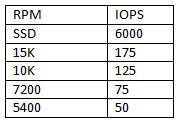
However, rather than working through a formula for your individual disks, there are a number of resources available that outline average observed IOPS values for a variety of different kinds of disks. For ease of calculation, use these values unless you think your own disks will vary greatly for some reason.
Below I list some of the values I've seen and used in my own environment for rough planning purposes. As you can see, the values for each kind of drive don't radically change from source to source.


Note : SSDS  IOPS = 6000

Sources:

• http://blog.aarondelp.com/2009/10/its-now-all-about-iops.html
• http://www.yellow-bricks.com/2009/12/23/iops/
• http://www.tomshardware.com/forum/251893-32-raid-raid

Note: The drive type doesn't enter into the equation at all. Sure, SAS disks will perform better than most SATA disks, but that's only because SAS disks are generally used for enterprise applications due to their often higher reliability as proven through their mean time between failure (MTBF) values. If a vendor decided to release a 15K RPM SATA disk with low latency and seek time values, it would have a high IOPS value, too.

Multidisk arrays

Enterprises don't install a single disk at a time, so the above calculations are pretty meaningless unless they can be translated to multidisk sets. Fortunately, it's easy to translate raw IOPS values from single disk to multiple disk implementations; it's a simple multiplication operation. For example, if you have ten 15K RPM disks, each with 175 IOPS capability, your disk system has 1,750 IOPS worth of performance capacity. But this is only if you opted for a RAID-0 or just a bunch of disks (JBOD) implementation. In the real world, RAID 0 is rarely used because the loss of a single disk in the array would result in the loss of all data in the array.
Let's explore what happens when you start looking at other RAID levels.

The IOPS RAID penalty

Perhaps the most important IOPS calculation component to understand lies in the realm of the write penalty associated with a number of RAID configurations. With the exception of RAID 0, which is simply an array of disks strung together to create a larger storage pool, RAID configurations rely on the fact that write operations actually result in multiple writes to the array. This characteristic is why different RAID configurations are suitable for different tasks.
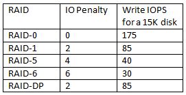
For example, for each random write request, RAID 5 requires many disk operations, which has a significant impact on raw IOPS calculations. For general purposes, accept that RAID 5 writes require 4 IOPS per write operation. RAID 6's higher protection double fault tolerance is even worse in this regard, resulting in an "IO penalty" of 6 operations; in other words, plan on 6 IOPS for each random write operation. For read operations under RAID 5 and RAID 6, an IOPS is an IOPS; there is no negative performance or IOPS impact with read operations. Also, be aware that RAID 1 imposes a 2 to 1 IO penalty.
The chart below summarizes the read and write RAID penalties for the most common RAID levels.

Parity-based RAID systems also introduce other additional processing that result from the need to calculate parity information. The more parity protection you add to a system, the more processing overhead you incur. As you might expect, the overall imposed penalty is very dependent on the balance between read and write workloads.
A good starting point formula is below. This formula does not use the array IOPS value; it uses a workload IOPS value that you would derive on your own or by using some kind of calculation tool, such as the Exchange Server calculator.
(Total Workload IOPS * Percentage of workload that is read operations) + (Total Workload IOPS * Percentage of workload that is read operations * RAID IO Penalty)
Source: http://www.yellow-bricks.com/2009/12/23/iops/
As an example, let's assume the following:

• Total IOPS need: 250 IOPS
• Read workload: 50%
• Write workload: 50%
• RAID level: 6 (IO penalty of 6)

Result: You would need an array that could support 875 IOPS to support a 250 IOPS RAID 6-based workload that is 50% writes.
This could be an unpleasant surprise for some organizations, as it indicates that the number of disks might be more important than the size (i.e., you'd need twelve 7,200 RPM, seven 10K RPM, or five 15K RPM disks to support this IOPS need).

The transport choice

It's also important to understand what is not included in the raw numbers: the transport choice -- iSCSI or Fibre Channel. While the transport choice is an important consideration for many organizations, it doesn't directly impact the IOPS calculations. (None of the formulas consider the transport being used.)
If you want more proof that the iSCSI/Fibre Channel choice doesn't necessarily directly impact your IOPS calculations, read this article on NetApp's site.
The transport choice is an important one, but it's not the primary choice that many would make it out to be. For larger organizations that have significant transport needs (i.e., between the servers and the storage), Fibre Channel is a good choice, but this choice does not drive the IOPS wagon.

Summary

In order to intricately understand your IOPS needs, you need to know a whole lot, including specific disk technicalities, your workload breakdown as a function of read vs. write, and the RAID level you intend to use. Once you implement your solution, you can use tools that are tailor-made to IOPS analysis, such as Iometer, to get specific, real-time performance values. This assumes that you have a solution in place that you can measure.

Oracle - Manual DB Create

Create Directory
-----------------
mkdir -p /apps/oracle/test

Crate a pfile with Min requirements
-----------------------------------
vi $ORACLE_HOME/dbs/initada.ora
db_name = ada
diagnostic_dest='/apps/oracle/test/'
control_files='/apps/oracle/test/ctrl1','/apps/oracle/test/ctrl2'
db_create_file_dest='/apps/oracle/test/'
db_create_online_log_dest_1='/apps/oracle/test/'
db_recovery_file_dest='/apps/oracle/test/'
db_recovery_file_dest_size=10G
diagnostic_dest='/apps/oracle/test/'

Create DB now
-------------------------------------
export ORACLE_SID=ada
sqlplus /nolog
STARTUP NOMOUNT
CREATE DATABASE ada
   USER SYS IDENTIFIED BY sys_password
   USER SYSTEM IDENTIFIED BY system_password
   LOGFILE GROUP 1 ('/apps/oracle/test/redo01.log') SIZE 10M,
           GROUP 2 ('/apps/oracle/test/redo02.log') SIZE 10M,
           GROUP 3 ('/apps/oracle/test/redo03.log') SIZE 10M
   MAXLOGFILES 5
   MAXLOGMEMBERS 5
   MAXLOGHISTORY 1
   MAXDATAFILES 100
   CHARACTER SET US7ASCII
   NATIONAL CHARACTER SET AL16UTF16
   EXTENT MANAGEMENT LOCAL
   DATAFILE '/apps/oracle/test/system01.dbf' SIZE 325M REUSE
   SYSAUX DATAFILE '/apps/oracle/test/sysaux01.dbf' SIZE 325M REUSE
   DEFAULT TABLESPACE users
      DATAFILE '/apps/oracle/test/users01.dbf'
      SIZE 500M REUSE AUTOEXTEND ON MAXSIZE UNLIMITED
   DEFAULT TEMPORARY TABLESPACE tempts1
      TEMPFILE '/apps/oracle/test/temp01.dbf'
      SIZE 20M REUSE
   UNDO TABLESPACE undotbs
      DATAFILE '/apps/oracle/test/undotbs01.dbf'
      SIZE 200M REUSE AUTOEXTEND ON MAXSIZE UNLIMITED
/

create spfile
------------------------
create spfile from pfile;

Create Dictonary Objects
-------------------------
cd $ORACLE_HOME/rdbms/admin

SQL> @catalog.sql
SQL> @catproc.sql
SQL> @pupbld.sql

Change Mode
--------------------------
Change Database Mode from NO-ARCHIVELOG to ARCHIVELOG.
SQL> shutdown immediate;
Database closed.
Database dismounted.
ORACLE instance shut down.
SQL> startup mount
ORACLE instance started.
Total System Global Area 150667264 bytes
Fixed Size 1331740 bytes
Variable Size 92278244 bytes
Database Buffers 50331648 bytes
Redo Buffers 6725632 bytes
Database mounted.
SQL> alter database ARCHIVELOG;
Database altered.
SQL> alter database OPEN;
Database altered.
Craete password File
--------------------
orapwd file=$ORACLE_HOME/dbs/orapwada entries=30


Thanks
Adarsh Kumar
AK Technosoft Corp.
www.aktechnosoft.com

Oracle - 12c New Features

Oracle12c New Features

 

SQL:

• Increased size limit for VARCHAR2, NVARCHAR2, and RAW datatypes to 32K  (from 4K).
• We can make a column invisible.
  SQL> create table test (column-name column-type invisible);
  SQL> alter table table-name modify column-name invisible;
  SQL> alter table table-name modify column-name visible;
• Oracle Database 12c has new feature called "Identity Columns" which are auto-incremented at the time of insertion (like in MySQL).
  SQL> create table dept (dept_id number generated as identity, dept_name varchar);
  SQL> create table dept (dept_id number generated as identity (start with 1 increment by 1 cache 20 noorder), dept_name varchar);
• Temporary undo (for global temporary tables) will not generate undo.
• No need to shutdown database for changing archive log mode.
• Duplicate Indexes - Create duplicate indexes on the same set of columns. Till Oracle 11.2, if we try to create an index using the same columns, in the same order, as an existing index, we'll get an error. In some cases, we might want two different types of index on the same data (such as in a datawarehouse where we might want a bitmap index on the leading edge of a set of columns that exists in a Btree index).
• PL/SQL inside SQL: this new feature allows to use DDL inside SQL statements (i.e.: to create a one shot function)
• The object DEFAULT clause has been enhanced. Adding a column to an existing table with a default value (much faster with Oracle 12c and it consumes less space than before, pointer to the Oracle Data Dictionary), applies also to sequences, identity types etc...
• Pagination query, SQL keywords to limit the number of records to be displayed, and to replace ROWNUM records.
  select ... fetch first n rows only;
  select ... offset m rows fetch next n rows only;
  select ... fetch first n percent rows only;
  select ... fetch first n percent rows with ties;
• Moving and Renaming datafile is now ONLINE, no need to put datafile in offline.
•  
• The TRUNCATE command has been enhanced with a CASCADE option which follows child records.
• Reduces contents of regular UNDO, allowing better flashback operations.

PL/SQL:

• PL/SQL Unit Security - A role can now be granted to a code unit. That means you can determine at a very fine grain, who can access a specific unit of code.
• SQL WITH Clause Enhancement - In Oracle 12c, we can declare PL/SQL functions in the WITH Clause of a select statement.
• Implicit Result Sets - create a procedure, open a ref cursor, return the results. No types, not muss, no mess. Streamlined data access (kind of a catch up to other databases).
• MapReduce in the Database - MapReduce can be run from PL/SQL directly in the database.
• We can use Booleans values in dynamic PL/SQL. Still no Booleans as database types.

Database:

• New background processes - LREG (Listener Registration), SA (SGA Allocator), RM

• Oracle Database 12c Data Pump will allow turning off redo for the import operation (only).
• Enhanced statistics (Hybrid histograms for more than 254 distinct values, dynamic sampling up to eleven, and stats automatically gathered during load).
• Row pattern matching - "MATCH_RECOGNIZATION" (identification of patterns within a table ordered/sorted by the SQL statement).
• Adaptive execution plans (change of the plan at runtime).
• Oracle 12c includes database level redaction, allowing granular control of access to sensitive data.
• Oracle introduced parameter PGA_AGGREGATE_LIMIT which is a real/PGA memory limit.
• UNDO for temporary tables can now be managed in TEMP, rather than the regular UNDO tablespace.

• Oracle Enterprise Manage Express (lightweight EM Cloud Control 12c version), replaces the Oracle Database console and, is installed automatically.
• Reduces the size of redo associated with recovering the regular UNDO tablespace.

ASM: (Oracle Grid Infrastructure new features)

• Introduction of Flex ASM, ASM would run only on 3 instances on a cluster even if more than 3, the instances that not have an ASM would request remote ASM, typically like SCAN. In normal conditions in a node if ASM fails the entire node will be useless, where in 12c the ability to get the extent map from remote ASM instance makes the node useful.
• Introduction of Flex Cluster, with light weight cluster stack, leaf node and traditional stack hub node, application layer is the typical example of leaf nodes where they don't require any network heartbeat.

RMAN:

• RMAN TABLE Point-In-Time Recovery (combination of Data Pump and RMAN, auxiliary instance required).
• Running SQL commands in RMAN without SQL keyword.
• Recover or copy files from Standby databases. 

Refresh a single datafile on the primary from the standby (or standby from primary).

• Table level restoration i.e object level.
• Incremental recovery more faster, many of the tasks removed.
• Rolling forward/Synchronizing a standby database.

Partitioning:

• Partitioning enhancements (partition truncate, cascading, global index cleanup, online moving of a partition, ...)
• Multiple partition operations in a single DDL.
• Interval-Ref Partitions - we can create a ref partition (to relate several tables with the same partitions) as a sub-partition to the interval type.
• Cascade for TRUNCATE and EXCHANGE partition.
• Asynchronous Global Index maintenance for DROP and TRUNCATE. Command returns instantly, but index cleanup happens later.
• Online move of a partition(without DBMS_REDEFINTIION).

Patching:

• Centralised patching.
• We can test patches on database copies, rolling patches out centrally once testing is complete.

Compression:
Automated compression with heat map.

Optimisation can be run on live databases with no disruption. Data optimization will monitor the data usage and with policy archive old data and hot data will be compressed for faster access. Inactive data can be more aggressively compressed or archived, greatly reducing storage costs.

Advanced Row compression (for Hot Data).
Columnar Query compression (for Warm Data).
Columnar Archive compression (for Archive Data).

Data Guard:

Oracle Database 12c introduces a new redo transportation method which omits the acknowledgement (to primary) of the transaction on the standby. This feature is called "Fast Sync" redo transport.

Creating a new type of redo destination called "Far Sync Standby". A "Far Sync Standby" is composed only of the standby control files, the standby redo logs and some disk space for archive logs which shall be sent to the Standby database. Failover & Switchover operations are totally transparent as the "Far Sync Standby" cannot be used as the target.

Data Guard Broker commands have been extended. The "validate database" command to checks whether the database is ready for role transition or not.

Dataguard Broker now supports cascaded standby.

 

Global Temporary Tables can now be used on an Active Guard standby database.

Pluggable Databases:

In Oracle 12c, in a pluggable database environment, we can create a single database container, and plug multiple databases into this container. All these databases then share the exact same oracle server/background processes and memory, unlike the previous versions where each database has its own background processes and shared memory. This helps in database consolidation and reduces the overhead of managing multiple desperate databases.

Container Database (CDB): Are the core data dictionary objects that come after an Oracle database installation.
Pluggable Database (PDB): Data dictionary objects and data related to the application. We can have many PDB plugged into a single CDB.

A new admin role "CDB Administrator" has been introduced in Oracle 12.1 release databases.
Multiple databases can then share a master LGWR process, but have their own dedicated LGWR process within the container.

All Oracle database options/features are available on the PDB level.

RMAN backup at CDB level.

We can unplug a PDB from a CDB to another CDB.
PDB's can be cloned inside the CDB.
Management of PDB (clone/creation/plug/unplug/drop) are implemented as SQLs.
Extremely fast PDB-provisioning (clone inside the CDB), because each CDB comes with a “PDB Seed”.
Database patch/upgrade management very quick as CDB is a single point of installation.
Each PDB has its own data dictionary.
Data Guard configuration on CDB as whole.
RMAN point-in-time recovery at PDB level (while other PDB's remains open).
Resource Manager is extended for creating, unplugging, plugging in, and cloning, dropping or even setting up for the open mode of the PDB.
Flashback of a PDB should be available for Oracle 12c Release 2.

Entire containers can be backed up in single run, regardless of how many databases they contain.
Upgrade one container database and all pluggable databases are upgraded.

New Commands
create pluggable database ...
alter pluggable database ...
drop pluggable database ...

New Views/Packages in Oracle 12c Release1

dba_pdbs
v$pdbs
cdb_data_files
dbms_pdb
dbms_qopatch